# Interactions in Linear Regression {#sec-example-regression-interactions}
Does an additional hour of studying have the same association with test scores for every study method? An **interaction** lets that slope differ between groups; here we fit and interpret one using only base R.
## Generate Example Data
These are synthetic scores for 120 students. We deliberately build in a steeper study-hours slope for the workshop group, then add random noise.
Each row of `students` represents one student. `runif()` draws study hours between one and nine, while `rep()` assigns 60 rows to each method. `factor()` tells R that the method is a category, not a numeric measurement. `set.seed()` makes the random draws reproducible when you rerun the example.
```{r}
#| label: ex-interaction-data
set.seed(2026)

students <- data.frame(
  hours = runif(120, min = 1, max = 9),
  method = factor(
    rep(c("Self-study", "Workshop"), each = 60),
    levels = c("Self-study", "Workshop")
  )
)

students$hours_centered <- students$hours - 5
workshop <- as.numeric(students$method == "Workshop")

students$score <- 65 +
  3 * students$hours_centered +
  4 * workshop +
  2 * students$hours_centered * workshop +
  rnorm(120, mean = 0, sd = 3)
```
With R's default treatment coding, the first factor level, `Self-study`, is the reference group. Subtracting five makes `hours_centered = 0` mean **five hours of studying**, not zero hours.
For example, two hours becomes -3 and eight hours becomes 3. Centering changes where we interpret the intercept and group difference; it does not change the fitted predictions when both predictors and their interaction remain in the model.
The `workshop` variable is 0 for self-study and 1 for workshop students. That makes the score-generation rule easier to follow:
- Self-study students have an expected score of 65 at five hours, with three additional points per extra hour.
- Workshop students have four additional points at five hours and an hourly slope that is two points steeper: five rather than three.
- `rnorm()` adds normally distributed noise with mean 0 and standard deviation 3, so students do not all fall exactly on these lines. The fitted coefficients will therefore differ somewhat from the values we used to generate the data.
## Fit the Interaction
In an R model formula, `hours_centered * method` includes both predictors **and** their interaction: `hours_centered + method + hours_centered:method`. There is no need to create a product column yourself.
The `~` separates the outcome, `score`, from the predictors. Using only `hours_centered + method` would allow different group intercepts but require the same hourly slope in both groups. Using `*` allows the slopes to differ too.
```{r}
#| label: ex-interaction-model
interaction_model <- lm(score ~ hours_centered * method, data = students)
coefficients <- coef(interaction_model)
round(coefficients, 2)
```
`lm()` fits the model, `coef()` extracts its named coefficient estimates, and `round()` changes only how we display them. Read these estimates as follows:
| Coefficient | Interpretation |
| --- | --- |
| `(Intercept)` | Predicted self-study score at five hours: `r round(coefficients["(Intercept)"], 2)` points. |
| `hours_centered` | Self-study slope: `r round(coefficients["hours_centered"], 2)` additional predicted points per extra hour. |
| `methodWorkshop` | Workshop minus self-study difference **at five hours**: `r round(coefficients["methodWorkshop"], 2)` points. |
| `hours_centered:methodWorkshop` | Workshop minus self-study **slope difference**: `r round(coefficients["hours_centered:methodWorkshop"], 2)` points per hour. |
The interaction coefficient is **not** the workshop slope. Add it to the self-study slope:
The `[["..."]]` expressions below retrieve individual coefficients by name. The interaction estimate is the amount we add to the reference group's slope, not a replacement for that slope.
```{r}
#| label: ex-interaction-slopes
self_study_slope <- coefficients[["hours_centered"]]
workshop_slope <- self_study_slope +
  coefficients[["hours_centered:methodWorkshop"]]

round(c("Self-study" = self_study_slope, "Workshop" = workshop_slope), 2)
```
An extra hour is associated with about `r round(self_study_slope, 2)` predicted points for self-study and `r round(workshop_slope, 2)` for workshop students. Neither coefficient is an overall slope averaged across both groups.
## Compare Predicted Scores
Use `predict()` to compare groups at specific hours. New data must use the **same centering value** as the training data.
Here, `expand.grid()` creates all six combinations of three study durations and two methods. These rows are scenarios, not additional observed students. `predict()` uses the fitted model to estimate a mean score for each scenario; it does not generate new random scores.
```{r}
#| label: ex-interaction-predictions
predictions <- expand.grid(
  hours = c(2, 5, 8),
  method = levels(students$method)
)
predictions$hours_centered <- predictions$hours - 5
predictions$predicted_score <- predict(interaction_model, newdata = predictions)

data.frame(
  hours = predictions$hours,
  method = predictions$method,
  predicted_score = round(predictions$predicted_score, 1)
)
```
Compare rows with the same hours: the workshop minus self-study difference changes as hours increase. The `methodWorkshop` coefficient describes that difference only at five hours, not at every study duration.
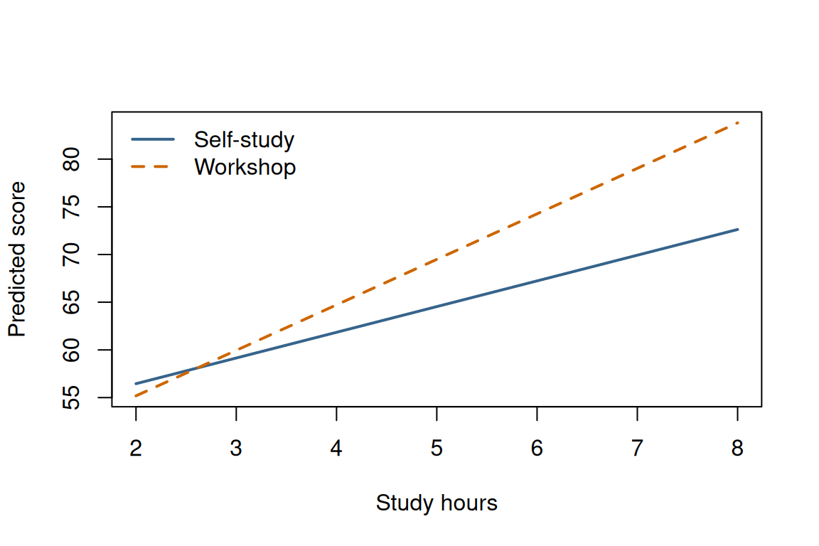
For example, at eight hours the predicted scores are `r round(predictions$predicted_score[predictions$hours == 8 & predictions$method == "Self-study"], 1)` for self-study and `r round(predictions$predicted_score[predictions$hours == 8 & predictions$method == "Workshop"], 1)` for the workshop. Their difference is about `r round(coefficients[["methodWorkshop"]] + 3 * coefficients[["hours_centered:methodWorkshop"]], 1)` points: the five-hour group difference plus three hours of the additional workshop slope.
To see that changing gap, `subset()` separates the prediction rows by method. `plot()` draws the self-study line, and `lines()` adds the workshop line to the same axes. Both lines come from our single interaction model, not separate regressions.
```{r}
#| label: ex-interaction-plot
#| fig-width: 6
#| fig-height: 4
#| fig-alt: "Two fitted score lines from two to eight study hours; the workshop line is steeper than the self-study line."
self_study_predictions <- subset(predictions, method == "Self-study")
workshop_predictions <- subset(predictions, method == "Workshop")

plot(predicted_score ~ hours, data = self_study_predictions,
     type = "l", col = "steelblue4", lwd = 2,
     ylim = range(predictions$predicted_score),
     xlab = "Study hours", ylab = "Predicted score")
lines(predicted_score ~ hours, data = workshop_predictions,
      col = "darkorange3", lwd = 2, lty = 2)
legend("topleft", legend = c("Self-study", "Workshop"),
       col = c("steelblue4", "darkorange3"), lwd = 2, lty = c(1, 2), bty = "n")
```
The different slopes show the fitted interaction. These are point estimates, not guaranteed individual scores or evidence that either method causes improvement. For uncertainty, `confint(interaction_model)` gives coefficient confidence intervals; the interaction interval concerns the **difference in slopes**.
For syntax, see the [R documentation for `lm()`](https://stat.ethz.ch/R-manual/R-devel/library/stats/html/lm.html); for interpretation, see [UCLA's interaction guide](https://stats.oarc.ucla.edu/r/seminars/interactions-r/).
<!-- shiny-app-builder:start -->
## Explore It with Shiny
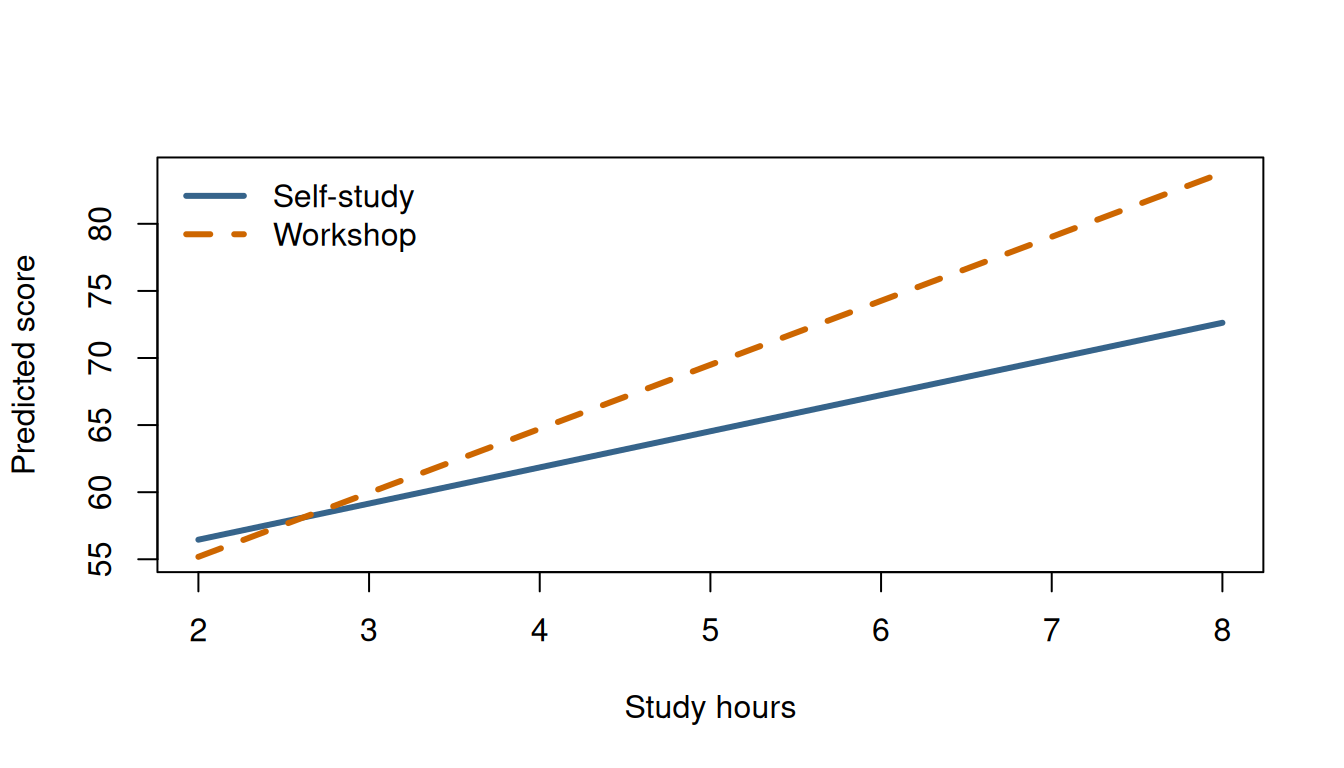
The companion app makes the page's central comparison adjustable: include the interaction to allow different fitted slopes, or remove it to require parallel slopes. You can also change the centering value, compare the methods at a selected number of study hours, and reveal the synthetic observations behind the lines.
```{r}
#| label: ex-interaction-shiny-preview-data
#| echo: false
shiny_preview_hour <- 8
shiny_preview_predictions <- subset(predictions, hours == shiny_preview_hour)
```
::: {.shiny-preview aria-labelledby="shiny-preview-title"}
<div class="shiny-preview-label" id="shiny-preview-title">Static preview</div>
<p class="shiny-preview-note">This shows the app's default state. The controls are intentionally disabled because the workshop page is not running a Shiny server.</p>
::: {.shiny-preview-layout}
::: {.shiny-preview-controls aria-label="Static representations of app controls"}
### Controls
<label for="shiny-preview-model">Model specification</label>
<select id="shiny-preview-model" disabled>
<option selected>Different slopes (interaction)</option>
<option>Parallel slopes (no interaction)</option>
</select>
<label for="shiny-preview-center">Center study hours at: <strong>5</strong></label>
<input id="shiny-preview-center" type="range" min="1" max="9" value="5" disabled>
<label for="shiny-preview-hour">Compare methods at: <strong>8 hours</strong></label>
<input id="shiny-preview-hour" type="range" min="1" max="9" value="8" disabled>
<label class="shiny-preview-check" for="shiny-preview-points">
<input id="shiny-preview-points" type="checkbox" disabled>
Show the synthetic student data
</label>
:::
::: {.shiny-preview-output}
### Fitted scores
```{r}
#| label: ex-interaction-shiny-preview-plot
#| echo: false
#| fig-width: 7
#| fig-height: 4
#| fig-alt: "Static app preview with a workshop fitted line that is steeper than the self-study fitted line from two to eight study hours."
plot(predicted_score ~ hours, data = self_study_predictions,
type = "l", col = "steelblue4", lwd = 3,
ylim = range(predictions$predicted_score),
xlab = "Study hours", ylab = "Predicted score")
lines(predicted_score ~ hours, data = workshop_predictions,
col = "darkorange3", lwd = 3, lty = 2)
legend("topleft", legend = c("Self-study", "Workshop"),
col = c("steelblue4", "darkorange3"), lwd = 3,
lty = c(1, 2), bty = "n")
```
<div class="shiny-preview-summary" aria-label="Default app results">
<div class="shiny-preview-stat shiny-preview-stat-self">
<span>Self-study slope</span>
<strong>`r round(self_study_slope, 2)`</strong>
<small>points per hour</small>
</div>
<div class="shiny-preview-stat shiny-preview-stat-workshop">
<span>Workshop slope</span>
<strong>`r round(workshop_slope, 2)`</strong>
<small>points per hour</small>
</div>
</div>
At eight hours, the fitted scores are **`r round(shiny_preview_predictions$predicted_score[shiny_preview_predictions$method == "Self-study"], 1)`** for self-study and **`r round(shiny_preview_predictions$predicted_score[shiny_preview_predictions$method == "Workshop"], 1)`** for the workshop.
:::
:::
:::
[Download the complete Shiny app](downloads/example-linear-regression-interactions-shiny.zip){download="example-linear-regression-interactions-shiny.zip"}
After extracting the ZIP, install `shiny` if needed, open R in the extracted `example-linear-regression-interactions` folder, and run:
```{r}
#| eval: false
shiny::runApp()
```
The app runs locally and does not use an API or upload data. Like the example above, it uses synthetic observations and illustrates fitted associations rather than causal effects. The app intentionally omits confidence intervals so the interaction and centering interpretations remain the focus.
<!-- shiny-app-builder:end -->